In my previous post, I cracked open the black box of machine learning with SHAP (SHapley Additive exPlanations) values, explaining how they break down a model’s prediction to its elemental parts for a single data point – this is what we call local interpretation.

If you haven’t read the first post, I highly recommend you start there. It provides the foundational explanation of what SHAP values are and how to calculate them for a single prediction. Understanding those basics will make the examples and insights in this follow-up much clearer.

Local explanations are just one piece of the puzzle. SHAP has a second, equally powerful feature: it can explain the model's reasoning at a global level. Sometimes, we need to zoom further out. What if you want to know which features your model generally cares about most? Or if certain predictors consistently dominate the decision process?

This is where global SHAP explanations come in. Rather than scrutinizing a single prediction, global SHAP analysis offers a big-picture view of how your model behaves across the entire dataset.

In this post, I explore this concept by using a small, easy-to-understand example from insurance premium modeling. As actuaries, this is often the level we need to work at to ensure model governance, align with regulatory expectations and communicate findings across teams.

From Local to Global

Imagine watching a movie one frame at a time. That's how local SHAP works. Now imagine watching the entire movie to understand its themes: that’s global SHAP. When you calculate SHAP values for each record in your data, it helps you figure out which features matter the most and spot important trends.

A Simplified Insurance Example

Understanding global SHAP lies in mean absolute SHAP values. This measure calculates the average size of a feature's effect on every prediction. Larger numbers show the feature holds more power. To fully understand global SHAP values, I will now extend our step-by-step approach to a mini example consisting of three policyholders. I will calculate local SHAP values for each one and then aggregate them to derive global SHAP values.

Assume we have a model trained with three features:

- X1: Age of driver - X2: Number of prior accidents - X3: Insurance score

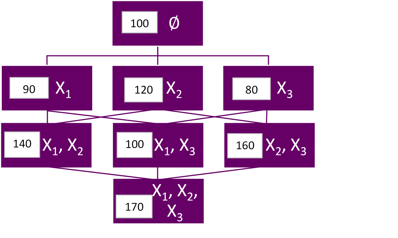
Here are the predictions made by the model for different combinations of features and policyholders. Each policyholder has their own prediction values for each subset of features.

Policyholder 1:

Policyholder 2:

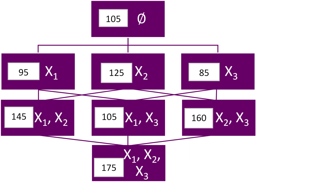
Policyholder 3:

Step 1: Compute Local SHAP Values for Each Policyholder

Policyholder 1

SHAP(X2) = (1/3)*(120 - 100 + 140 - 90 + 160 - 80) = (1/3)*(20 + 50 + 80) = 50

SHAP(X1) = (1/3)*(90 - 100 + 140 - 120 + 100 - 80) = (1/3)*30 = 10

SHAP(X3) = (1/3)*(80 - 100 + 100 - 90 + 160 - 120) = (1/3)*30 = 10

Policyholder 2

SHAP(X2) = (1/3)*(130 - 110 + 150 - 100 + 165 - 95) = (1/3)*(20 + 50 + 70) = 46.67

SHAP(X1) = (1/3)*(100 - 110 + 150 - 130 + 110 - 95) = (1/3)*25 = 8.33

SHAP(X3) = (1/3)*(95 - 110 + 110 - 100 + 165 - 130) = (1/3)*30 = 10

Policyholder 3

SHAP(X2) = (1/3)*(125 - 105 + 145 - 95 + 160 - 85) = (1/3)*(20 + 50 + 75) = 48.33

SHAP(X1) = (1/3)*(95 - 105 + 145 - 125 + 105 - 85) = (1/3)*30 = 10

SHAP(X3) = (1/3)*(85 - 105 + 105 - 95 + 160 - 125) = (1/3)*30 = 10

Step 2: Compute Global SHAP Values (Average Across Policyholders)

SHAP(X2) = (50 + 46.67 + 48.33) / 3 = 48.33

SHAP(X1) = (10 + 8.33 + 10) / 3 = 9.44

SHAP(X3) = (10 + 10 + 10) / 3 = 10

The global SHAP values reveal that X2 is the most influential feature, contributing an average of 48.33 units to the model’s predictions across all observations. In comparison, X1 and X3 have much smaller average contributions, at 9.44 and 10, respectively. This suggests that the model relies most heavily on X2 when making predictions, while X1 and X3 play more moderate roles. Understanding this hierarchy of feature importance helps us validate the model’s behavior and ensures alignment with domain knowledge or regulatory expectations.

In summary, this blog’s example demonstrates how you can move from granular explanations (local SHAP) to an overall understanding (global SHAP) by simply averaging the impact of each variable across many predictions. This technique gives actuaries a powerful lens into how models behave across the entire portfolio.

Why Global SHAP Values Matter for Actuaries

From an actuarial perspective, global SHAP values serve multiple functions:

• Model validation: Confirm that your model aligns with expected domain model behaviors (e.g., prior accidents matter more than age)
• Governance and transparency: Satisfy internal and regulatory stakeholders with feature-level summaries
• Communication: Translate technical model behavior into intuitive summaries for business leaders and non-technical audiences

In pricing, underwriting, or claims analytics, global SHAP offers a defensible, quantifiable way to describe what your model is doing, without needing to open the algorithm itself.

Looking Ahead: Beyond Feature Importance

SHAP can do more than rank variables. For example:

• SHAP dependence plots show how a feature’s effect changes across its values and in combination with others, thus allowing you to examine complex interactions up close.
• You might discover, for example, that insurance scores matter only for drivers without prior accidents on their record - a signal of interaction.
• These findings can influence how you set underwriting and pricing rules, and ensure that your model isn't just guessing.

In my next post, I will explore these topics further, in addition to digging into SHAP’s limitations and what it takes to put explainability into practice on a large scale.